LaserLab Analyzer
User's Guide: An Intelligent Computational Platform for Multi-Scale Modeling of Laser–Matter Interactions
Legal Notice
LaserLab Analyzer is an original scientific software platform developed at the Department of Physics, University of Tlemcen. All source code, physical models, material databases, and documentation are protected under copyright law. Unauthorized reproduction, distribution, or modification of any part of this software is strictly prohibited. Academic use for research and educational purposes is permitted provided that appropriate attribution is given.
© 2026 Tires Soulef Selssabil, Zeyneb Bedrane, and Bereksi Reguig Adil Acheraf. All rights reserved.
1. Introduction
1.1 Purpose of This Guide
This guide describes the theoretical foundations, software architecture, and operational workflow of LaserLab Analyzer v1.0. It is intended for researchers, engineers, and graduate students who apply laser processing simulations in photonics, materials science, or industrial micromachining. The document is organized so that new users can follow the workflow sequentially, while experienced users may consult individual chapters as reference material.
1.2 Scope and Capabilities
LaserLab Analyzer provides deterministic, physics-based simulation of pulsed laser interactions with solid targets across three temporal regimes — nanosecond (ns), picosecond (ps), and femtosecond (fs) — and three material classes: metals, semiconductors, and dielectrics. The platform integrates:
- A multi-regime physical modeling engine covering thermal, ultrafast, and phase-transition phenomena.
- A structured thermophysical and optical material database with validated internal consistency.
- Quantitative prediction of ablation threshold, heat-affected zone (HAZ), temperature field, and material state evolution.
- An AI-based interpretation module that translates numerical outputs into structured scientific reports and process recommendations.
1.3 Dual-Use Intent
The platform is designed for two primary contexts. In academic and educational settings, it supports training in laser–matter interaction physics, parameter sensitivity studies, and regime comparison. In industrial contexts, it serves as a decision-support tool for process optimization, ablation threshold prediction, and laser micromachining planning.
1.4 Document Structure
Chapter 2 defines the nomenclature and physical parameters used throughout the guide. Chapter 3 presents the platform architecture. Chapters 4–6 detail the physical models implemented for each temporal regime and material class. Chapter 7 describes the AI interpretation engine. Chapter 8 traces the complete simulation workflow. Chapter 9 documents output quantities, and Chapter 10 provides the reference list.
2. Nomenclature
2.1 Laser Parameters
| Symbol | Quantity | SI Unit |
|---|---|---|
| λ | Wavelength | nm |
| τ | Pulse duration | s |
| E | Pulse energy | J |
| F | Laser fluence | J m⁻² |
| I | Laser intensity | W m⁻² |
| f_r | Repetition rate | Hz |
| w₀ | 1/e² beam radius at focus | μm |
| F_th | Ablation threshold fluence | J m⁻² |
2.2 Material and Thermal Properties
| Symbol | Quantity | SI Unit |
|---|---|---|
| ρ | Mass density | kg m⁻³ |
| C_p | Specific heat capacity | J kg⁻¹ K⁻¹ |
| k | Thermal conductivity | W m⁻¹ K⁻¹ |
| α_th | Thermal diffusivity (= k/ρC_p) | m² s⁻¹ |
| δ | Optical penetration depth (= 1/α) | m |
| α | Absorption coefficient | m⁻¹ |
| R | Surface reflectivity | — |
| n, κ | Complex refractive index components | — |
| T_m, T_b | Melting & Boiling temperature | K |
| L_f, L_v | Latent heats of fusion and vaporization | J kg⁻¹ |
2.3 Two-Temperature Model (TTM) Parameters
| Symbol | Quantity | SI Unit |
|---|---|---|
| T_e, T_l | Electron & Lattice temperature | K |
| C_e, C_l | Electron & Lattice heat capacity | J m⁻³ K⁻¹ |
| k_e | Electron thermal conductivity | W m⁻¹ K⁻¹ |
| g | Electron–phonon coupling constant | W m⁻³ K⁻¹ |
| τ_ep | Electron–phonon relaxation time | s |
2.4 Carrier and Plasma Dynamics
| Symbol | Quantity | SI Unit |
|---|---|---|
| N, N_cr | Free carrier & Critical plasma density | m⁻³ |
| D | Ambipolar diffusion coefficient | m² s⁻¹ |
| τ_r | Carrier recombination time | s |
| G | Carrier generation rate | m⁻³ s⁻¹ |
| E_g | Bandgap energy | eV |
| γ | Keldysh parameter | — |
| W_MPI | Multiphoton ionization rate | m⁻³ s⁻¹ |
| W_tunnel | Tunnel ionization rate | m⁻³ s⁻¹ |
| σ_k | k-photon absorption cross-section | m²ᵏ s⁻¹ J⁻ᵏ |
2.5 Derived Output Quantities
| Symbol | Quantity | SI Unit |
|---|---|---|
| T(x,t) | Spatiotemporal temperature field | K |
| l_th | Thermal diffusion length | m |
| L_HAZ | HAZ depth | m |
| L_abl | Ablation depth per pulse | m |
| S(z,t) | Volumetric laser energy source term | W m⁻³ |
3. Platform Architecture
3.1 Design Principles
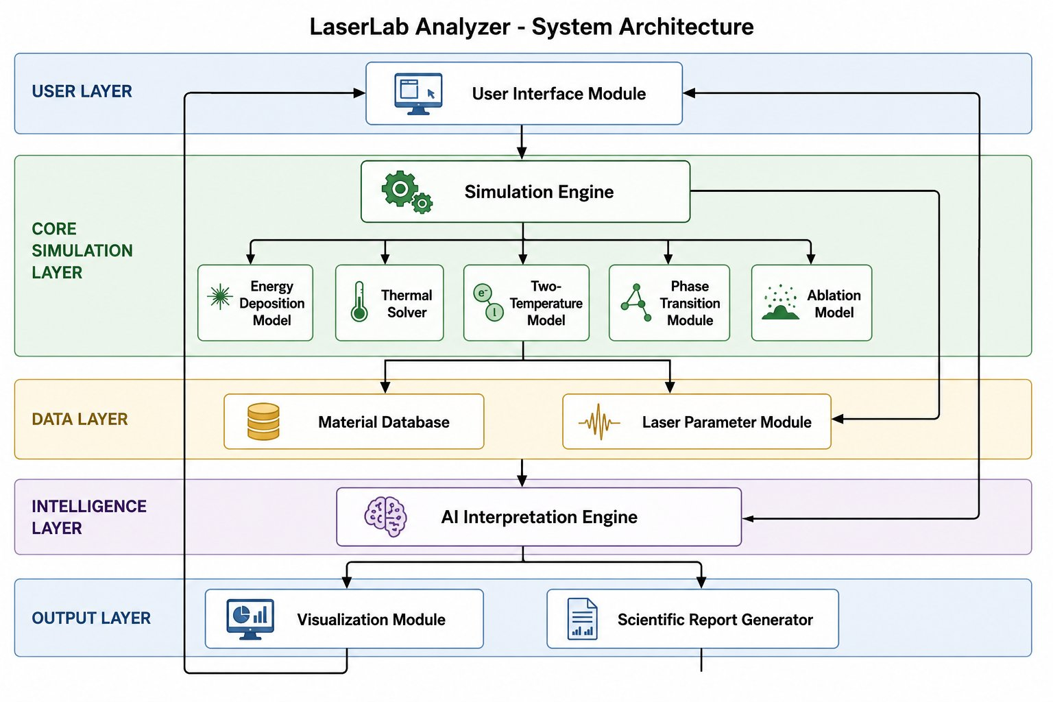
LaserLab Analyzer is built around a layered modular architecture governed by the principles of high cohesion and low coupling, consistent with best practices in scientific software design. Each layer exposes well-defined interfaces, allowing individual modules to be updated or extended without affecting the rest of the platform. The system is deterministic: given identical inputs, it produces identical outputs, which is a necessary condition for reproducible scientific computation.
3.2 Layer Description
| Layer | Module | Primary Responsibilities |
|---|---|---|
| Presentation | UserInterfaceModule | Parameter input, material selection, result visualization and export |
| Simulation Core | SimulationEngine | Energy deposition, heat transport, TTM, phase transitions, ablation evaluation |
| Data | MaterialDatabaseModule / LaserParameterModule | Thermophysical and optical property retrieval; laser parameter validation and fluence computation |
| Intelligence | AIInterpretationEngine | Automated analysis, regime classification, and scientific report generation |
| Output | OutputVisualizationModule | Temperature maps, ablation curves, HAZ profiles, and exportable data files |
3.3 Module Interface Specifications
3.3.1 UserInterfaceModule
This module acts as the central hub for user interaction. It securely captures user inputs—such as specific laser configurations and material choices—and routes them to the underlying processing layers. Once the simulation and analysis are complete, this layer is responsible for taking the complex data and rendering it back to the user in an accessible, visual, and easily digestible format.
3.3.2 SimulationEngine
This is the physical heart of the platform. It is a highly adaptable computational engine that models exactly how laser energy is absorbed and how heat travels through a given material over time. Without exposing its internal mechanics, this engine automatically selects the correct physical laws based on the laser's pulse duration (handling everything from long nanosecond pulses to ultrafast femtosecond interactions). It computes the resulting physical phenomena, including extreme temperature spikes, structural melting or vaporization, and the final depth and rate of material removed (ablation).
3.3.3 Data Layer Modules
The data layer is split into two specialized modules that feed verified constants into the simulation:
Material Database Module: An isolated, secure repository containing all the necessary thermal, physical, and optical constants for various materials. It operates independently to guarantee that the simulation core is always fed consistent and scientifically accurate material properties.
Laser Parameter Module: A dedicated validation checkpoint for the laser settings. It ensures that the user's chosen laser characteristics (such as energy, duration, and wavelength) are physically coherent. It also acts as a gatekeeper, verifying that the selected laser settings mathematically align with the physics models the simulation core intends to use.
3.3.4 AIInterpretationEngine
Rather than just handing raw numbers back to the user, this advanced module acts as an automated scientific analyst. It reviews the raw physical data produced by the Simulation Core, identifies key behavioral regimes, and translates complex numerical outcomes into comprehensive, human-readable analytical reports and insights.
3.3.5 Visualization Layer
This module is strictly responsible for data translation and export. It takes the raw matrices and data arrays from the simulation and transforms them into clear graphical representations—such as heatmaps, affected zone profiles, and physical deformation curves—while also packaging the raw data into standard formats for the user to download and use elsewhere.
4. Physical Foundations
4.1 Governing Time Scales
The physical response of a material to pulsed laser irradiation is determined primarily by the relationship between the pulse duration τ and the characteristic times governing electron–lattice relaxation, thermal diffusion, and hydrodynamic motion.
| Physical Process | Characteristic Time Scale |
|---|---|
| Electron thermalization | 10 – 100 fs |
| Electron–phonon energy coupling | 1 – 10 ps |
| Free-carrier recombination | 1 ps – 1 ns |
| Thermal diffusion into the bulk | 1 ns – 1 μs |
| Hydrodynamic plume expansion | > 10 ps |
4.2 Temporal Regime Classification
Three distinct interaction regimes are identified according to the pulse duration relative to the electron–phonon coupling time τ_ep:
| Regime | Pulse Duration | Condition | Dominant Physics |
|---|---|---|---|
| Nanosecond | τ ~ 10⁻⁹ s | τ ≫ τ_ep | Thermal equilibrium; strong diffusion; melting and vaporization |
| Picosecond | τ ~ 10⁻¹² s | τ ~ τ_ep | Partial electron–lattice decoupling; mixed thermal/electronic response |
| Femtosecond | τ ~ 10⁻¹⁵ s | τ ≪ τ_ep | Strong non-equilibrium; electronic energy deposition; ultrafast ablation |
4.3 Thermal Diffusion Length
The spatial extent of the heat-affected zone is characterized by the thermal diffusion length: l_th = √(α_th · τ).
Two limiting cases determine the nature of the interaction:
• l_th ≫ δ → Strong thermal diffusion dominates (ns regime); extensive HAZ formation.
• l_th ≪ δ → Thermal confinement (fs regime); energy remains localized near the surface; minimal collateral damage.
4.4 Laser Energy Deposition
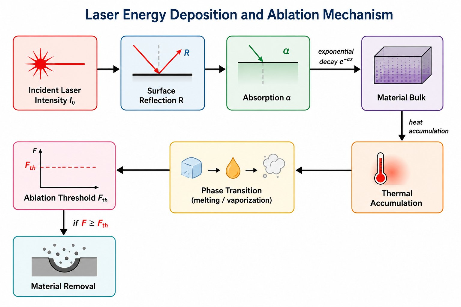
In all regimes, the volumetric energy source term is derived from Beer–Lambert attenuation modified by surface reflectivity:
S(z, t) = α (1 − R) I₀(t) exp(−α z)
where α is the linear absorption coefficient, R is the surface reflectivity, I₀(t) is the time-dependent surface intensity, and z is the depth coordinate measured from the irradiated surface. The optical penetration depth is δ = 1/α.
4.5 Material Classes and Optical Response
| Material Class | Representative Examples | Primary Absorption Mechanism |
|---|---|---|
| Metals | Al, Cu, Ti, steel alloys | Intraband/interband absorption; high reflectivity in the visible and near-IR |
| Semiconductors | Si, GaAs, Ge | Interband absorption controlled by E_g; carrier-mediated heating |
| Dielectrics | SiO₂, fused silica, ceramics | Transparent below bandgap; nonlinear multiphoton and tunnel ionization |
5. Nanosecond Regime
In the nanosecond regime (τ ≫ τ_ep), electrons and the lattice remain in mutual thermal equilibrium throughout the pulse duration. Heat diffusion governs the temperature evolution; the dominant material responses are melting, vaporization, and, at sufficiently high fluence, hydrodynamic plume expansion.
5.1 Metals — Heat Diffusion Equation
Temperature evolution in a metallic target is governed by the classical Fourier heat equation:
ρ C_p ∂T/∂t = ∇ ·(k ∇ T) + S(z, t)
with S(z,t) as defined previously. Because l_th ≫ δ, heat diffuses well beyond the absorption zone, generating a large HAZ. The HAZ depth scales as L_HAZ ~ √(α_th · τ). At moderate fluence, the one-dimensional ablation depth per pulse is approximated by L_abl = δ · ln(F / F_th), where F_th is the ablation threshold fluence.
5.2 Semiconductors — Carrier Generation and Diffusion
Above-gap irradiation generates free electron–hole pairs through interband absorption. Their density N evolves according to the ambipolar diffusion equation:
∂N/∂t = G − N/τ_r + D ∇²N
where G is the carrier generation rate driven by photon absorption, τ_r is the recombination time, and D is the ambipolar diffusion coefficient. The generated carriers thermalize rapidly and subsequently transfer energy to the lattice via phonon emission, driving conventional thermal ablation.
5.3 Dielectrics — Multiphoton Ionization and Optical Breakdown
Wide-bandgap dielectrics are transparent at the fundamental laser frequency. Ionization is initiated through multiphoton absorption: for a k-photon process, the ionization rate scales as W_MPI = σ_k · I^k, where σ_k is the k-photon absorption cross-section. Once a seed electron density is established, avalanche ionization amplifies it exponentially. When N reaches the critical plasma density N_cr, the material undergoes optical breakdown, characterized by localized melting, microcracking, and thermal damage. The long pulse duration allows significant heat diffusion during the ionization cascade, resulting in a comparatively large damage zone.
6. Picosecond and Femtosecond Regimes
6.1 The Two-Temperature Model
When the pulse duration is comparable to or shorter than the electron–phonon coupling time, the electron subsystem can no longer be described by a common temperature with the lattice. The Two-Temperature Model (TTM), originally formulated by Anisimov et al. (1974), captures this non-equilibrium state through two coupled partial differential equations:
Electron subsystem: C_e(T_e) ∂T_e/∂t = ∇·(k_e ∇T_e) − g (T_e − T_l) + S(z, t)
Lattice subsystem: C_l ∂T_l/∂t = g (T_e − T_l)
where g is the electron–phonon coupling constant, C_e(T_e) is the temperature-dependent electron heat capacity, and k_e is the electron thermal conductivity. The source term S(z,t) appears only in the electron equation, as photon energy is absorbed directly by the electron gas.
6.2 Picosecond Regime
6.2.1 Metals: In the ps regime (τ ~ τ_ep), the TTM equations apply. Because energy transfer from electrons to the lattice is incomplete during the pulse, thermal diffusion is reduced compared to the ns case, yielding a smaller HAZ and higher processing precision.
6.2.2 Semiconductors: Carrier dynamics remain governed by ambipolar diffusion, but the shorter pulse allows less time for carrier diffusion. The result is a mixed physical response combining electronic excitation, transient non-equilibrium heating, and partial thermal ablation.
6.2.3 Dielectrics: Free-electron generation incorporates both multiphoton and avalanche ionization: dN/dt = W_MPI + β N I − N/τ_r. Optical breakdown is partial and diffusion-limited, yielding improved machining precision.
6.3 Femtosecond Regime
6.3.1 Metals: The thermal confinement condition strictly holds. The laser pulse deposits energy exclusively into the electron gas before appreciable energy transfer to the lattice occurs (T_e ≫ T_l). After the pulse ends, electron–phonon coupling drives rapid lattice heating, triggering non-thermal ablation via Coulomb or phase explosion.
6.3.2 Semiconductors: Carrier generation is dominated by strong-field nonlinear ionization. The Keldysh parameter γ determines whether multiphoton (γ > 1) or tunnel ionization (γ < 1) governs.
6.3.3 Dielectrics: All ionization channels contribute simultaneously. When N ≥ N_cr, the material forms an overdense plasma and the interaction transitions to a strongly absorbing, confined regime, enabling subwavelength modification volumes with negligible peripheral thermal damage.
6.4 Regime Comparison
| Property | ns | ps | fs |
|---|---|---|---|
| Thermal equilibrium | Yes | Partial | No |
| Thermal diffusion extent | Strong | Moderate | Negligible |
| HAZ size | Large | Intermediate | Minimal |
| Dominant ablation mechanism | Thermal | Mixed | Electronic / non-thermal |
| Melting contribution | Dominant | Partial | Weak or absent |
| Achievable machining precision | Low | High | Ultrahigh |
| Model implemented | Fourier HDE | TTM + carrier eq. | Ultrafast TTM + Keldysh |
7. AI Interpretation Engine
7.1 Role and Scope
The AI Interpretation Engine is a post-processing subsystem that operates on the numerical outputs of the SimulationEngine and translates them into structured scientific commentary and engineering recommendations. It is not a surrogate model: it does not replace physical computation but augments it with automated semantic analysis.
7.2 Input Data
The engine receives spatiotemporal temperature fields, ablation depth, material removal efficiency, HAZ dimensions, phase fraction evolution, the complete laser configuration, and the material property set.
7.3 Functional Outputs
Based on this input set, the engine produces regime classification, detection of nonlinear effects and threshold transitions, comparative analysis, structured scientific reports, and process optimization recommendations.
8. Simulation Workflow
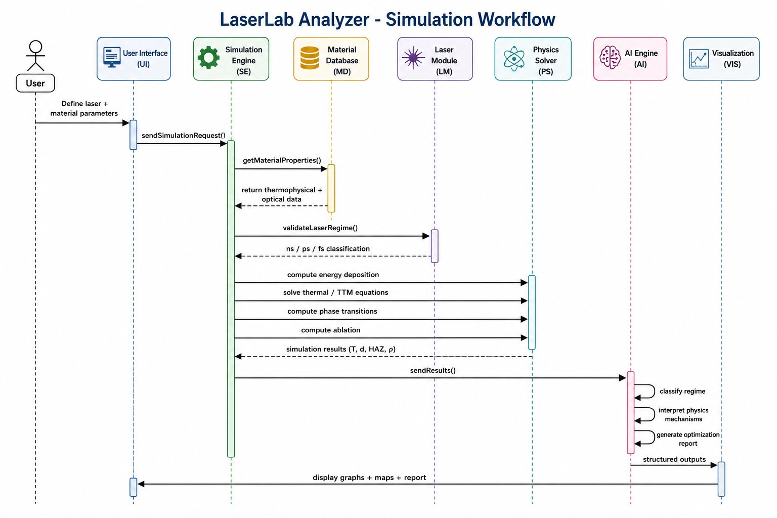
The following sequence describes the complete computational pipeline from user input to final report generation.
| Step | Action | Responsible Module |
|---|---|---|
| 1 | User specifies laser parameters and selects target material. | UserInterfaceModule |
| 2 | Validates the parameter set and infers the temporal regime (ns/ps/fs). | LaserParameterModule |
| 3 | Retrieves the complete property set for the selected material. | MaterialDatabaseModule |
| 4 | Selects the appropriate physical model (Fourier HDE, TTM, or ultrafast TTM + Keldysh) based on the regime. | SimulationEngine |
| 5 | Computes the volumetric source term S(z,t). | EnergyDepositionModel |
| 6 | Integrates the governing equations forward in time. | ThermalSolver / UltrafastDynamicsSolver |
| 7 | Evaluates melting, vaporization, and ablation criteria at each time step. | PhaseTransitionModule |
| 8 | Computes ablation depth per pulse and cumulative material removal. | AblationModel |
| 9 | Assembles temperature maps, ablation curves, HAZ profiles, and phase data. | OutputVisualizationModule |
| 10 | Analyzes the full output set and generates the structured scientific report. | AIInterpretationEngine |
9. Output Quantities and Post-Processing
| Output Module | Computed Quantities | Primary Use |
|---|---|---|
| Ablation Characteristics | Threshold fluence F_th, ablation rate, material removal efficiency | Process parameter selection; ablation window identification |
| Thermal Field | Temperature distribution T(x,t), thermal diffusion length l_th, heat accumulation | HAZ assessment; thermal fatigue evaluation |
| Heat-Affected Zone | HAZ depth, lateral extension, thermal gradient distribution | Collateral damage estimation; precision benchmarking |
| Material State Evolution | Phase fractions (solid/liquid/vapor), density evolution, thermodynamic state variables | Phase transition characterization; melt pool analysis |
9.1 Temperature Field
The temperature field T(x,t) is computed on a one-dimensional spatial grid extending from the irradiated surface into the bulk. Results are rendered as spatiotemporal maps and time-series profiles at user-selected depths.
9.2 Ablation Metrics
Ablation depth per pulse is computed using the regime-appropriate model: the logarithmic law for the ns case, or modified forms accounting for non-equilibrium energy deposition in the ps and fs regimes.
9.3 Heat-Affected Zone
HAZ dimensions are extracted from the computed temperature field by applying a threshold criterion corresponding to either the onset of microstructural modification or the melting temperature.
9.4 AI-Generated Report
The AI Interpretation Engine report is appended automatically to each simulation output. It includes a regime identification statement, a summary of dominant physical mechanisms, quantitative result highlights, and process recommendations.
10.Boundary Conditions and Adaptive Mesh Refinement
10.1 Boundary Condition Formulations
The governing equations are closed by boundary conditions at the irradiated surface (z = 0) and at the far-field boundary (z → ∞ or z = L). Three canonical formulations are used:
10.1.1 Neumann Boundary Condition (Heat Flux)
The laser source term enters the domain as a prescribed heat flux at the irradiated surface. At the far-field boundary, an insulating (zero-flux) condition is applied when the simulation domain is sufficiently deep relative to the thermal diffusion length.
10.1.2 Dirichlet Boundary Condition (Fixed Temperature)
When the target is thermally anchored (e.g., a substrate held at fixed temperature by a heat sink), the far-field condition is prescribed as T(z = L, t) = T_amb. This is appropriate for thin-film targets.
10.1.3 Robin Boundary Condition (Convective / Radiative Loss)
For simulations that include convective cooling at the irradiated surface or substrate face, the mixed (Robin) condition is applied. This formulation is most relevant in the ns regime at elevated fluence where surface temperatures approach or exceed boiling.
10.1.4 TTM Interface Coupling (Electron–Phonon Boundary)
In the TTM formulation, the interface between the electron and lattice subsystems at z = 0 is treated as an internal coupling condition. This condition ensures energy conservation at the electron subsystem boundary and prevents unphysical temperature discontinuities.
10.2 Adaptive Mesh Refinement
To resolve sharp spatial gradients that develop near the ablation front and in the plasma formation zone without incurring the computational cost of a uniformly fine global mesh, LaserLab Analyzer implements an Adaptive Mesh Refinement (AMR) strategy based on local gradient criteria.
10.2.1 Refinement Criteria
Mesh refinement is triggered when the normalized gradient of a monitored field variable exceeds a user-defined threshold θ_ref. Two field variables are monitored by default: Plasma or free-carrier density gradient, and Temperature gradient.
10.2.2 Refinement Strategy
The mesh is refined locally by halving the cell size in regions satisfying either criterion, up to a user-specified maximum refinement level. Coarsening is applied in the far-field region where gradients are negligible. The default refinement threshold is θ_ref = 0.1.